Computing error bars for velocity.
The computation of error bars is based on the scatter of the points
plotted in the bvasqc.ps file. Consider an alternative X-Y
plot of points about a linear trend, where the ``x'' values are
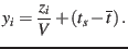
the depths,  , of each geophone station, and the ``y''
values are pseudo arrival times computed from the bvas solution
velocity and relative time shifts,
, of each geophone station, and the ``y''
values are pseudo arrival times computed from the bvas solution
velocity and relative time shifts,  , about the mean shift,
 ,
,
 |
(8) |
The slope of a least squares linear fit to these pseudo times,  , would correspond to the slowness, 1/V. The problem is to then estimate
the variance in the reciprocal of the slope of linear solution. That
is, if
, would correspond to the slowness, 1/V. The problem is to then estimate
the variance in the reciprocal of the slope of linear solution. That
is, if  , then we solve for the variance,
 , assuming a least squares solution to the problem. For N pairs of
(x,y), we can write the velocity as the reciprocal of the least squares
solution for the slope of the line as
, assuming a least squares solution to the problem. For N pairs of
(x,y), we can write the velocity as the reciprocal of the least squares
solution for the slope of the line as
![$\displaystyle V=\frac{1}{m}=\frac{\left[\left(\sum x_{i}\right)^{2}-N\sum\left(...
...(\sum x_{i}\right)\left(\sum y_{i}\right)-N\sum\left(x_{i}y_{i}\right)\right]}.$](img47.png) |
(9) |
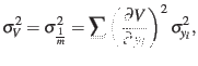
The variance of the velocity,
 , is given by
 |
(10) |
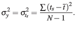
where
 is assumed a constant for all and
is estimated by the scatter around the mean . In other words,
is given by
is assumed a constant for all and
is estimated by the scatter around the mean . In other words,
is given by
 |
(11) |
After some algebra, we find that,
![$\displaystyle \sigma_{V}^{2}=\sigma_{\frac{1}{m}}^{2}=\sigma_{t_{s}}^{2}\cdot\f...
...m x_{i}\right)\left(\sum y_{i}\right)-N\sum\left(x_{i}y_{i}\right)\right]^{4}}.$](img52.png) |
(12) |
This permits us to treat the semblance determined velocity, V, as
though it were the result of a least squares fit to picked arrival
times, and thus obtain an estimate of the uncertainty in the phase
velocity determination. The velocity error bars are computed as the
square root of
 (units of m/s). These error bars
may be scaled by 1.96 to obtain an estimate of the 95% confidence
interval (assuming normally distributed errors). The unscaled values
are output to the file bvas.his, and then later used in the
Octave joint inversion, cainv3.m, to obtain confidence limits
on both stiffness,
(units of m/s). These error bars
may be scaled by 1.96 to obtain an estimate of the 95% confidence
interval (assuming normally distributed errors). The unscaled values
are output to the file bvas.his, and then later used in the
Octave joint inversion, cainv3.m, to obtain confidence limits
on both stiffness,  and damping,
  .
.
pm
2018-04-08