Delay Time Method

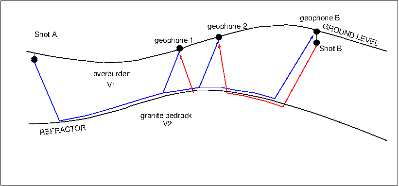
The basic theory can be found in many engineering seismology text books. The following is a brief summary of how BSU implements the method. A highly simplified case is shown in Figure 32

Figure 32: Simplified delay time setup. Shots A and B shoot into geophones 1 and 2.

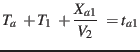
The delay time equation for Shot A to geophone 1 is given by

$$T_a ~+ T_1 ~ + \dfrac{X_{a1}}{V_2}~=t_{a1}$$ (24)

where $T_a$ is the delay time at shot A, $T_1$ is the delay time at geophone 1, $X_{a1}$, is the horizontal distance between shot A and geophone 1, and $t_{a1}$ is the observed travel time from shot A to geophone 1. The refractor velocity is $V_2$. A complete system becomes, in matrix form, the following:

$$G \centerdot m = d$$ (25)

or

$$\left[ \begin{array}{ccccc} 1 & 0 & 1 & 0 & X_{a1}\\ 1 & 0 & 0 & ... ...[\begin{array}{c} t_{a1}\\ t_{a2}\\ t_{ab}\\ t_{b1}\\ t_{b2}\end{array} \right]$$ (26)

Equation 24 is the first row of equation 26. Matrix $G$ is constructed by a program, bref, such that the first columns correspond to the shots, the other columns the geophones, ending in a last column giving the distance between a shot and receiver.