The delaytm.m procedure solves for the delay times, and then
resolves them into two end-limit solutions. Variations in delay times
are resolved totally into a variation in the refractor structure with
the formula
 |
(38) |
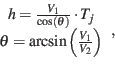
where  is the j-th delay time and ``h'' is the distance
from the source or geophone to the refractor. This distance, h, is
a radius specifying a circle, somewhere on which the refractor may
be found. In delaytm.m, the refractor position is plotted a distance,
h, directly below the source or geophone (unmigrated position). For
the purpose of most engineering surveys, migration of the refractor
point is not a significant issue (the distances are quite small).
is the j-th delay time and ``h'' is the distance
from the source or geophone to the refractor. This distance, h, is
a radius specifying a circle, somewhere on which the refractor may
be found. In delaytm.m, the refractor position is plotted a distance,
h, directly below the source or geophone (unmigrated position). For
the purpose of most engineering surveys, migration of the refractor
point is not a significant issue (the distances are quite small).
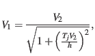
The alternative end-limit resolution of delay times is as a variation
in overburden velocity. The user provides a distance from the recording
surface to the refractor (held constant), and an overburden velocity
is found from the formula
 |
(39) |
where is the j-th delay time and ``h'' is the constant
distance from the recording surface to the refractor. This assumes
that the refractor velocity,  , is constant, and the only
variation is in
, is constant, and the only
variation is in  , the overburden velocity. This type of solution
makes sense when the water content of the overburden soil is known
to vary, and the overburden thickness is relatively constant. In reality,
the truth will be somewhere between these two limiting cases. See
Michaels (9) for a discussion on this topic.
, the overburden velocity. This type of solution
makes sense when the water content of the overburden soil is known
to vary, and the overburden thickness is relatively constant. In reality,
the truth will be somewhere between these two limiting cases. See
Michaels (9) for a discussion on this topic.
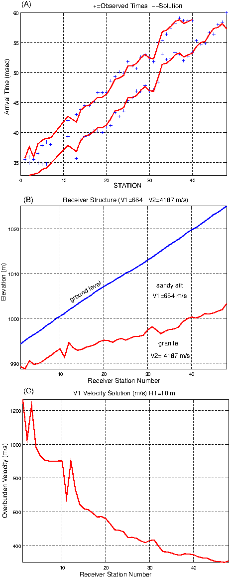
One should probably produce xfig
scaled plots, as some CAD work is usually required to clean things
up. Figure 37 shows how a final merging of the exported *.fig files
will look with a little CAD effort. In this case, the structural solution,
Figure 37B is preferred
because of our knowledge of the geology from trenching and surface observations.
Figure 37:
Line 3 solution, merged xfig plots. A). Arrival times and fit, B). Structural Solution (accepted), C). Overburden velocity solution (rejected)
|
 |
pm
2018-04-08