Next: Spectral Analysis of Surface Up: Surface Wave Processing Previous: Example Rayleigh Wave Processing: Contents Index
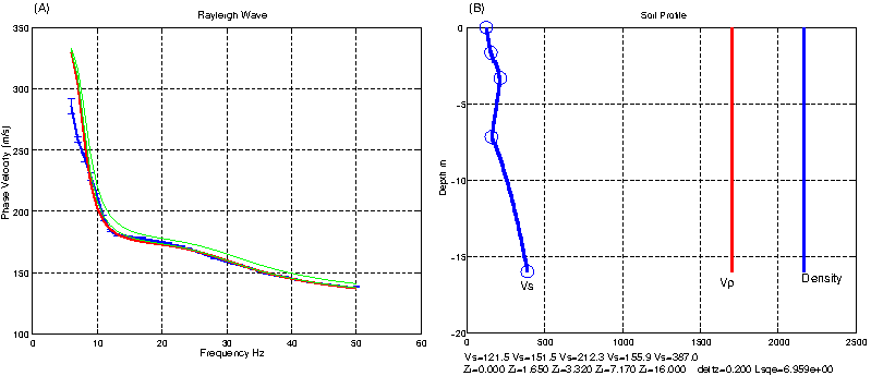
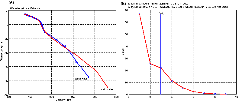
The program, invR1.m, will attempt to determine a layered model which matches a measured phase velocity dispersion profile. As in program, FwdR1.m, the dispersion curve is read from a text file, bvax.his. The Fortran subroutine, rwv.f, must also be in the directory. The inversion ran for 3 iterations. The solution is shown graphically in Figure 47. Only 3 singular values were used (see Figure 48).
 |
 |
pm 2018-04-08