Example of bnfd
The program bnfd uses a design BSEGY data file to set up the
details of the synthetic data set (number of traces, sample interval,
layout of source relative to receivers, etc). In this example, we
will use the lambv.seg file from the second lamb example
(section 7.1.1.4 above). It does not matter what components
are specified in the design file, since this will be ignored in bnfd
(which uses command line arguments to specify the source and receiver
polarizations). The sample shown in Figure 54 is for a horizontal
force (in  direction) and observer stations located at the
same elevation as the source, extending in a line out to 48 meters.
The motion captured at the observer point is also in the
direction (we would not expect any motion in the other directions).
The command used to generate this sample is
direction) and observer stations located at the
same elevation as the source, extending in a line out to 48 meters.
The motion captured at the observer point is also in the
direction (we would not expect any motion in the other directions).
The command used to generate this sample is
bnfd lambv.seg 1 433. 250. 1700. 100. 50. 1 7
The material properties are the same as for the Lamb's problem example.
However, this solution is in a whole space, and we are observing the
computation of body waves, free from any boundary.
Figure 54:
Near and Far Field computations (source in x1, motion in x1 directions).
The data have been trace qualized by the L2 norm of each offset signal to prevent
fading of the motion due to amplitude decay.
|
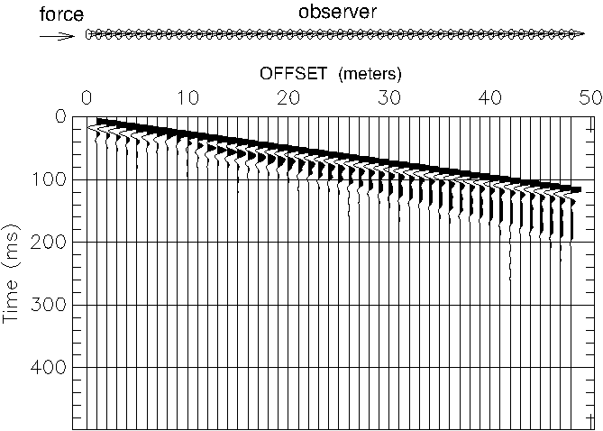 |
The near field dominates at the near offsets, and then declines in
amplitude with increasing offset. The listing file produced by bnfd
(in this case bnfdlamb.lst) provides a listing of the relative
amplitudes. The S-wave amplitude is zero in this case, and we are
only looking at P- and Near-field waves. A sample of the amplitudes
taken from the listing are:
- Offset=1 meter, Near Field=9.362e-05 P-wave= 2.497e-10
- Offset=24 meters, Near Field=6.772e-09 P-wave=1.040e-11
- Offset=48 meters, Near Field=8.465e-10 P-wave= 5.201e-12
So we can see that we have not yet gone far enough out for the P-wave
to match the near field wave amplitude. The source wavelet in this
case had a center frequency of 50 Hz, and a decay rate of 100 per
second.
pm
2018-04-08