Next: From Displacement to Velocity Up: Synthetic Rayleigh Wave Seismograms Previous: Editing the waves.d file Contents Index
The computed synthetic seismograms are for particle displacement. Thus, they are not what one would see with a velocity geophone (which measures particle velocity). The source wavelet is captured in a text file from the waves run. The file is named m0.mat. It consists of 2 columns, record time and signal amplitude. This wavelet is filtered by the computed Rayleigh wave earth response and computed radiation pattern of the source moment tensor to produce the synthetic.
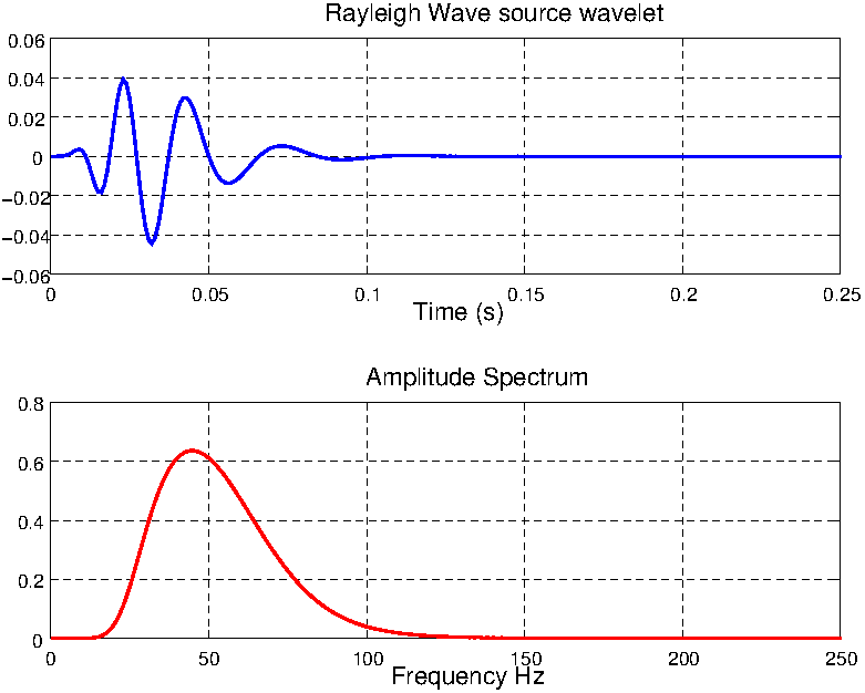
The actual spectral bandwidth will be less than is commonly defined (common definitions include the -3dB or -6dB point for example). We can plot the wavelet and its amplitude spectrum by running the Octave procedure, m0.m, generated by waves. For example, a brief listing of the generated m0.m file is shown below:
clear
 // generated by waves.f <pm@cgiss.boisestate.edu>
 // scalar source moment, plot wavelet

 data=[...
    0.00000   0.1145539E-06 ;...
    0.00100   0.1769859E-05 ;...
    0.00200   0.1318357E-04 ;...
    0.00300   0.6318095E-04 ;...
       *           *
       *           *
       *           *
    1.02100  -0.1863727E-42 ;...
    1.02200  -0.2017870E-42 ;...
    1.02300  -0.2087935E-42 ;...
 ];
 tm=data(:,1);
 mo=data(:,2);
 Mo=fft(mo);
 npts=length(mo);
 k=npts/2;
 dt=tm(2)-tm(1);
 frq=0:npts-1;
 frq=frq/(npts*dt);
 subplot(211)
 plot(tm,mo,'-b','linewidth',2);
 title('Rayleigh Wave source wavelet');
 xlabel('Time (s)');
 grid on;
 subplot(212)
 plot(frq(1:k),abs(Mo(1:k)),'-r','linewidth',2)
 title('Amplitude Spectrum');
 xlabel('Frequency Hz');
 grid on;
The resulting plot is shown in Figure 61. Note, that the bandwidth (by common definitions) is less than the values specified by fmin and fmax.
 |
pm 2018-04-08